Real-Time Analytics on Snowflake: Which BI Platform to Pick?

Snowflake is genuinely capable of sub-minute freshness now. Snowpipe Streaming on the high-performance architecture went generally available on AWS in September 2025 and on Azure in November 2025, with ingest-to-query latency typically under ten seconds. Dynamic tables refresh on a target lag as low as one minute. Hybrid tables push the floor toward sub-second for the workloads that need it.

The problem isn’t Snowflake. The problem is that most BI tools don’t surface what Snowflake actually delivers.

Every BI vendor in 2026 claims real-time. The marketing pages all say it, the demo videos all show it, and the analyst reports all rank it. None of them mean the same thing. A “real-time” Tableau dashboard refreshes its extract on a 15-minute schedule. A “real-time” Power BI report runs in Import mode against data pulled at 2 a.m. A “live” connection in one tool means the warehouse is queried on every interaction; in another tool it means a cached extract gets checked for staleness every fifteen minutes.

The honest question for a data platform lead evaluating BI on Snowflake is not which vendor’s marketing claims real-time. It’s where the freshness ceiling actually lives in your stack — and which BI tools respect it.

This article gives you a four-link mental model for thinking about that ceiling, names what each link contributes to your latency, maps the major BI platforms onto where they genuinely sit on the live-query versus extract spectrum, and gives you a POC checklist your data team can run in an afternoon to verify any vendor’s claims against your real Snowflake account.

TL;DR

• “Real-time on Snowflake” is a system property, not a tool feature. Your dashboard’s freshness equals the slowest link in a four-link chain: ingestion → warehouse processing → BI tool refresh → user view.
• Most teams optimize the BI tool layer when their actual ceiling lives in ingestion. Sub-minute freshness on Snowflake is achievable today with Snowpipe Streaming plus dynamic tables plus a live-query BI tool. Sub-second requires hybrid tables or a separate streaming layer.
• Astrato, Sigma, and Looker default to live-query architectures that surface Snowflake’s freshness directly. Tableau and Power BI default to extract or Import modes that add staleness; their live modes work but accept real trade-offs. ThoughtSpot’s behavior depends on which path you configure. Metabase varies with cache settings.

What “real-time on Snowflake” actually means

Three honest tiers are hiding inside the same word.

Real-time (sub-second). The dashboard reflects an event within milliseconds to a few seconds of it happening in the source system. Live trading floors, in-flight fraud detection, real-time bidding, sports betting odds. On Snowflake, this tier requires hybrid tables (Unistore) or a streaming analytics layer alongside Snowflake. Mainstream BI tools are not the right answer here, and no Snowflake-connected BI tool will deliver this on a standard analytical warehouse pattern.

Near-real-time (sub-minute). The dashboard reflects an event within five to sixty seconds of it landing in Snowflake. Operational dashboards, real-time inventory, fulfillment status, customer-facing usage analytics. This is what mainstream patterns deliver today: Snowpipe Streaming for ingestion, dynamic tables or raw tables for the queryable layer, and a live-query BI tool that doesn’t cache.

Fresh enough (5–15 minutes). The dashboard is current within the typical refresh interval of a batch pipeline. Most operational reporting, finance dashboards, marketing analytics, weekly business reviews. This is what most teams actually need, and it’s what most BI tool extract schedules are calibrated for.

The mistake most buyers make is conflating these tiers. A vendor demo shows a dashboard updating “in real-time” — usually meaning sub-minute on a curated dataset — and the buyer assumes that’s the right tier for their use case without asking whether sub-second matters or whether 15-minute would be fine. The right starting question is which tier your use case actually requires. The wrong starting question is which BI tool has the loudest real-time claim.

The four-link freshness chain

Your dashboard is only as fresh as the slowest link in the chain from source system to user view. Four links, in order. Each contributes its own latency. The ceiling is set by whichever one is slowest.

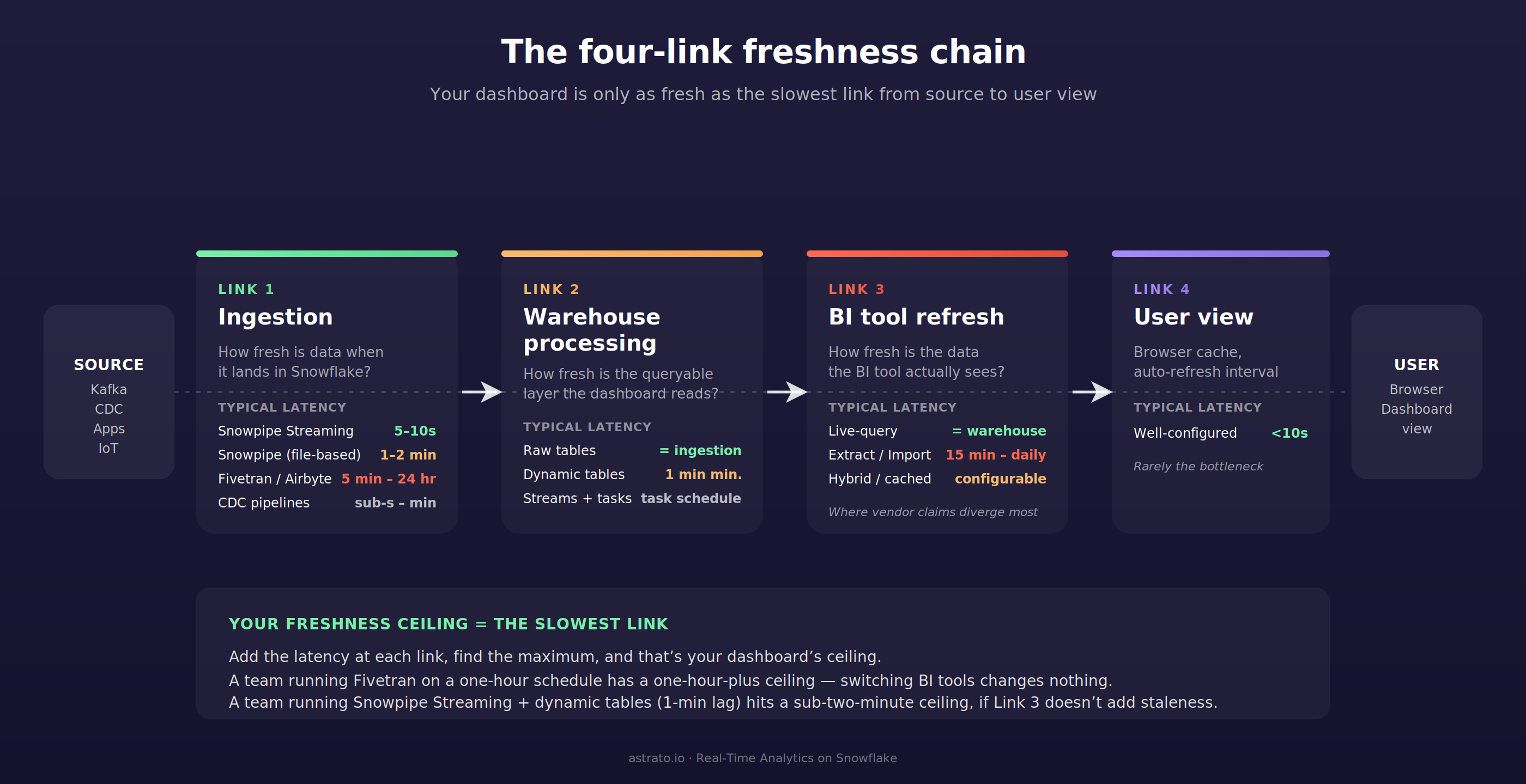
Link 1 — Ingestion latency. How fresh is the data when it lands in Snowflake?

This is the link most teams underestimate. Snowpipe Streaming on the high-performance architecture delivers ingest-to-query latency of approximately five to ten seconds per Snowflake’s documentation, and Cboe’s published implementation reports a P95 query latency under thirty seconds against a live ingested dataset. Classic Snowpipe (file-based, micro-batched) typically runs at one to two minutes from the time a file lands in cloud storage. Fivetran, Airbyte, and similar managed connectors run anywhere from five minutes to twenty-four hours depending on the connector and the configured sync frequency. CDC pipelines vary from sub-second to minutes depending on tooling.

If your pipeline is a Fivetran connector syncing every fifteen minutes, your real-time ceiling is fifteen minutes. No BI tool can give you fresher data than what’s in Snowflake, and no marketing claim about live-query architecture changes that.

Link 2 — Warehouse processing latency. How fresh is the data once it’s queryable in the form the dashboard needs?

Raw tables match ingestion freshness — whatever lands is what’s available. Dynamic tables refresh on a target lag with a minimum of one minute per Snowflake’s documentation, and target lag is a target rather than a guarantee. Streams plus tasks refresh on whatever schedule the task is configured for. Materialized views refresh automatically in the background, but with limitations on supported SQL.

The honest planning question is whether your dashboard reads raw tables or transformed ones. Reading raw tables eliminates Link 2 latency entirely; reading dynamic tables adds the target lag; reading materialized views or task-output tables adds whatever the refresh interval is. Many teams forget Link 2 exists because their pipeline diagrams show Snowflake as a single box. The Data Products on Snowflake article treats this layer in detail — the same warehouse-resident transformation logic that makes a data product clean is what makes a sub-minute dashboard possible.

Link 3 — BI tool refresh latency. How fresh is the data the BI tool actually sees?

Live-query architectures match the warehouse’s freshness exactly — every dashboard interaction issues a SQL query and the result reflects whatever Snowflake returns at that moment. Extract-based architectures pull a copy of the data on a schedule; the dashboard is as fresh as the last extract refresh. Hybrid architectures vary by configuration.

This is the link the article spends the most time on, because it’s the one buyers have the most control over and the most confusion about. It’s also the link where vendor marketing diverges most sharply from product reality.

Link 4 — User view latency. How fresh is the data the user actually sees?

Browser cache, dashboard auto-refresh interval, query result cache hits, the time between when the user loads the page and when they look at it. For any well-configured tool this is under ten seconds. It rarely matters except when teams set dashboard auto-refresh intervals of fifteen minutes and then complain that data is stale.

The mental model: add the latency at each link, find the maximum, and that’s your dashboard’s freshness ceiling. Optimizing a link below the ceiling buys you nothing. A team running Snowpipe-Streaming-fed dynamic tables with a one-minute lag has a sub-two-minute ceiling — switching from a tool with a 15-minute extract schedule to one with live-query gets them from sixteen minutes down to two. A team running a Fivetran connector on a one-hour schedule has a one-hour-plus ceiling, and switching BI tools changes nothing.

Most teams optimize Link 3 when their ceiling lives in Link 1.

The Snowflake side: what enables sub-minute freshness

Snowflake’s own architecture has caught up with sub-minute freshness in ways that didn’t exist three years ago. Four primitives matter for this conversation.

Snowpipe Streaming is Snowflake’s low-latency ingestion service. Rows land directly in Snowflake tables without staging files. The high-performance architecture supports up to 10 GB/s per table with ingest-to-query latency typically under ten seconds. Use cases include real-time analytics dashboards, log and event analysis, IoT telemetry, change-data-capture pipelines from operational databases, and live application events. The Kafka connector for Snowpipe Streaming flushes data within one second of buffer commit.

Dynamic tables are declarative materialized transformations that refresh on a target lag. Minimum target lag is one minute. The refresh process runs incrementally where the SQL pattern allows, full-refresh otherwise. Dynamic tables remove the operational burden of writing and scheduling tasks for transformation pipelines. The trade-off is that target lag is a target, not a guarantee — if a refresh takes longer than the lag setting, actual lag exceeds it.

Streams plus tasks are Snowflake’s older mechanism for building incremental pipelines. A stream tracks change data on a base table; a task runs SQL on a schedule and consumes the stream. More flexibility than dynamic tables, more operational overhead. Useful when dynamic tables’ SQL constraints don’t fit the transformation pattern.

Hybrid tables (Unistore) are Snowflake’s row-store-backed table type for transactional workloads. Sub-second point lookups, OLTP-style updates, and the same tables remain queryable from analytical workloads. The path to genuine sub-second freshness on Snowflake runs through hybrid tables, but they’re a different architecture choice than the analytical warehouse pattern most teams default to. For most BI use cases on Snowflake, hybrid tables are a sub-second escape hatch, not the standard pattern.

The combination most teams want for near-real-time is Snowpipe Streaming feeding raw tables, with dynamic tables (one-minute target lag) producing the queryable transformed layer, behind a live-query BI tool. End-to-end ceiling: roughly fifteen seconds at the ingestion link, one minute at the warehouse-processing link, sub-second at the BI tool link, sub-ten-seconds at the user view link. Total ceiling: under two minutes from event to dashboard.

That architecture is the answer to the source-of-truth question driving this article: yes, Snowflake can do sub-minute end-to-end. The constraint is on the BI side.

The BI tool side: live-query, extract, and the architectures in between

Three architectures, in order of how much latency they add to Link 3.

Live-query architecture issues a SQL query to Snowflake at the moment the user requests data. There’s no extract, no schedule, no synced copy. The dashboard’s freshness equals the warehouse’s freshness. The trade-offs are real and worth naming: every interaction triggers a warehouse query (concurrency and warehouse spin-up matter), there’s no caching layer to mask warehouse slowness, and per-query cost models favor warehouses that handle the load. Astrato, Sigma, and Looker default here.

Extract architecture pulls a snapshot of the data from Snowflake into the BI tool’s own engine on a schedule. Subsequent dashboard interactions query the extract, not the warehouse. The dashboard’s freshness equals the last extract refresh — fifteen minutes, an hour, daily, whatever the schedule says. The trade-off is the inverse: dashboards are fast for users, warehouse load is bounded, but data is stale by definition. Tableau defaults here. Power BI’s Import mode is functionally equivalent.

Hybrid architecture combines both: live queries for some interactions, extracts or caches for others. Behavior depends on configuration. Power BI’s DirectQuery, Sigma’s optional materialized data sets, ThoughtSpot’s choice between Falcon and live Snowflake, and Metabase’s per-question caching all sit here. The architectural answer to “is this tool real-time” is “depends on how you configured it.”

The marketing language that hides this is “live” — used loosely enough that it can mean any of the three. A vendor saying “live dashboards on Snowflake” might mean live-query (Link 3 latency = warehouse latency), live-connection (extracts disabled, queries pass through), or live-feeling (extracts refresh frequently enough that users perceive freshness). The honest distinction is whether the SQL Snowflake actually receives includes the user’s interaction in real time, or whether the BI tool is serving from its own copy.

The verifiable test is whether dashboard interactions appear in Snowflake’s query_history view in real time. If they do, you’re on a live-query architecture. If they don’t, you’re on an extract or cache.

The platforms that compete here

Each platform’s behavior on Snowflake depends on configuration. Here’s where each one defaults and what its actual freshness floor is in normal use.

Astrato — live-query, no extracts

Astrato is a warehouse-native BI platform built around live queries to Snowflake. Every chart, every dashboard, every interaction issues a SQL query to the warehouse at the moment the user requests data. There’s no extract layer, no scheduled refresh, no synced copy. The dashboard’s freshness equals Snowflake’s freshness, full stop. Astrato benefits from Snowflake’s result cache automatically — repeated queries with no underlying data change return instantly from cache without consuming warehouse compute, which is a cost benefit, not a freshness compromise.

The honest trade-off: Astrato doesn’t add a caching layer that would mask warehouse slowness. If a query is slow on Snowflake — large unclustered scan, cold warehouse spin-up, queue at peak concurrency — the dashboard reflects that. Some extract-based tools mask this with cached snapshots, which is a real benefit for some teams and use cases. The deliberate positioning is that Astrato delivers whatever freshness Snowflake delivers, no more and no less.

Best fit for: teams with an ingestion pipeline already delivering sub-minute freshness who want a BI tool that doesn’t add staleness below their actual ceiling. Strong fit for customer-facing analytics where end-customers expect to see their own activity live.

Sigma — live-query primarily, with optional materialization

Sigma defaults to a live-query architecture against Snowflake. Dashboard interactions compile to SQL and execute on the warehouse. Sigma also offers optional materialized data sets — pre-aggregated tables Sigma writes back to Snowflake — which add staleness when used but reduce warehouse compute for high-cardinality interactions. The architecture choice is per-element rather than platform-wide.

Best fit for: teams that want live-query as the default with the option to materialize specific high-cost elements. The dual-mode flexibility is a feature for some teams and a configuration-discipline problem for others.

Tableau — extracts by default, live connection as an alternative

Tableau’s default mode is the .hyper extract — a snapshot of the data pulled from Snowflake into Tableau’s in-memory data engine on a schedule. The minimum extract refresh interval on Tableau Cloud is fifteen minutes. Subsequent dashboard interactions query the extract, not Snowflake. This is fast for users and bounded in warehouse cost, but stale by definition.

Tableau’s live connection mode does exist and works against Snowflake. Every interaction issues a SQL query to the warehouse, with freshness equal to Snowflake’s. The trade-off named in Tableau’s own documentation: live connections are an expensive operation per query, and the same dashboard opened by ten users in different time zones runs ten times against the warehouse, which Snowflake’s result cache mitigates but doesn’t eliminate.

Best fit for: teams already invested in Tableau who can switch specific dashboards to live connections where freshness matters. Less ideal as the default architecture for sub-minute use cases.

Power BI — Import is the default; DirectQuery is the live mode

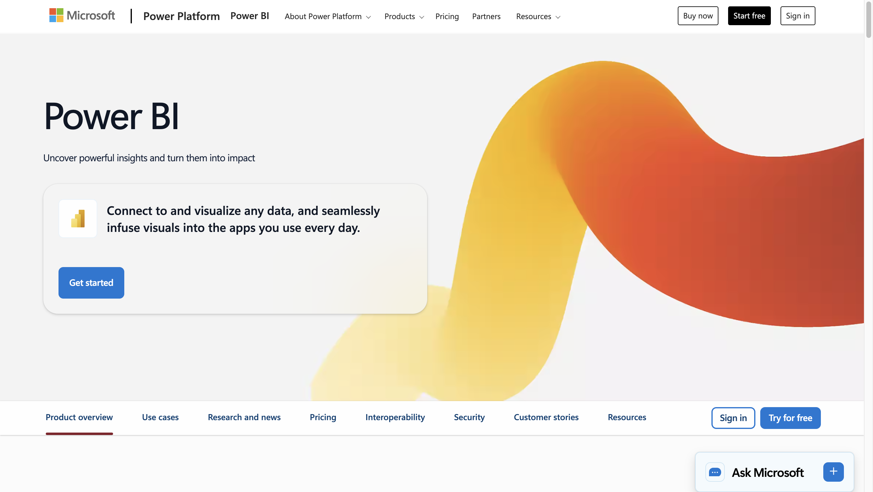
Power BI ships with two primary connectivity modes. Import pulls data from Snowflake on a refresh schedule and stores it in Power BI’s in-memory model; the dashboard queries the imported model, not Snowflake. DirectQuery issues SQL to Snowflake on every interaction, with freshness equal to the warehouse’s.

DirectQuery on Power BI has a documented constraint: queries that return more than one million rows from cloud sources fail with a “maximum allowed size” error, except in Premium capacity with admin-set limits. The limit applies to intermediate results, not final visuals, so high-cardinality columns combined with non-aggregated visuals can hit the ceiling unexpectedly. Microsoft’s own documentation recommends Hybrid tables (Power BI’s name for partitioned models combining DirectQuery for recent data and Import for historical) for teams that want Import speed on cold data and DirectQuery freshness on hot data.

Best fit for: organizations standardized on Power BI and Microsoft Entra ID who can structure their data model to fit DirectQuery’s constraints. Teams that default to Import mode are accepting their refresh schedule as their freshness ceiling.

Looker — live-query architecture with optional materialization

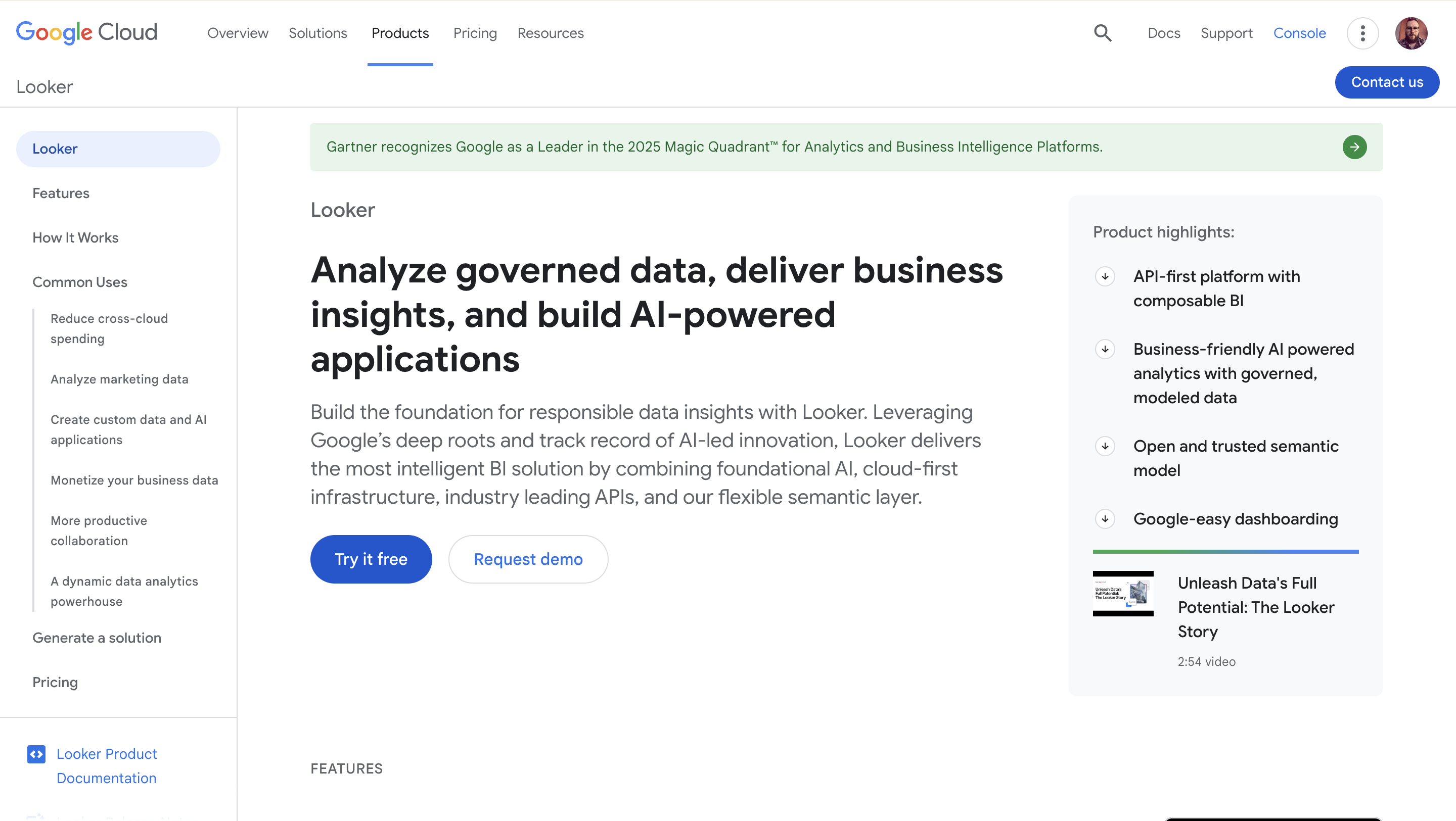
Looker’s LookML semantic layer compiles user interactions into SQL that executes against Snowflake at query time. There’s no native extract layer; the architectural default is live-query. Looker offers persistent derived tables (PDTs) — materialized intermediate results that Looker writes back to the warehouse and refreshes on a configurable trigger. PDTs introduce staleness for the queries that read them, but they’re an opt-in optimization rather than a default.

The trade-off is the LookML learning curve and the modeler-led development pattern. Teams that have invested in LookML get warehouse-native freshness with semantic-layer governance. Teams that haven’t built the LookML model are dependent on the data team to expose every new analytical view.

Best fit for: teams with mature LookML models who want live-query freshness without giving up semantic governance. The architectural fit on freshness is strong; the modeling investment is the cost of entry.

ThoughtSpot — two distinct architectures depending on which path you configure

ThoughtSpot supports two fundamentally different architectures against Snowflake. The first is Falcon, ThoughtSpot’s in-memory database — data is loaded from Snowflake into Falcon on a schedule, and dashboard interactions query Falcon, not Snowflake. The second is live Snowflake mode (called “linked” data in ThoughtSpot’s own docs) — interactions issue SQL to Snowflake and query the warehouse directly.

ThoughtSpot’s documentation is clear that linked data is slower than Falcon for interactive queries because ThoughtSpot doesn’t cache linked data. The trade-off is the inverse of every extract-based tool: live Snowflake gives you warehouse freshness at the cost of per-query latency; Falcon gives you in-memory speed at the cost of load-schedule staleness. Recent ThoughtSpot positioning emphasizes the live-Snowflake path, including integrations with Snowflake Interactive Analytics for sub-second performance on direct queries against Snowflake.

Best fit for: teams who explicitly choose the live Snowflake mode and accept the latency profile. Teams who default to Falcon are operating an in-memory architecture, not a warehouse-native one.

Metabase — live-query with configurable caching

Metabase issues SQL to Snowflake on dashboard interactions by default. Result caching is configurable per question, per dashboard, or globally. With caching off, freshness equals warehouse freshness. With caching on, freshness equals the cache TTL. There’s no native extract pipeline.

The architectural pattern is fine for internal analytics on smaller teams. The freshness story depends entirely on cache settings, which means it depends on the team’s discipline rather than the platform’s default. Teams that don’t actively manage cache configuration will end up with freshness that drifts from what the dashboards imply.

Best fit for: internal teams comfortable managing cache settings and willing to verify per-dashboard configuration. Less ideal for use cases where freshness consistency matters across a large dashboard estate.

The streaming-analytics tier — Materialize, Tinybird, RisingWave, Pinot-based tools like StarTree — sits in a separate category. These aren’t BI tools running on Snowflake; they’re streaming analytics layers that ingest from Kafka or a CDC source and deliver sub-second query latency on a continuously-updated materialized view. For genuine sub-second use cases (fraud detection in flight, real-time bidding, live trading dashboards), the right architectural answer is usually a streaming layer alongside Snowflake rather than a BI tool plus Snowflake. They’re worth knowing about when sub-second is a hard requirement; they’re not on the BI evaluation shortlist for most teams.

A worked example: real-time inventory on Snowflake

Inventory is the cleanest illustration of when this article’s pattern is the right answer. Sub-minute matters — you don’t want to oversell stock, mis-route a shipment, or surface a stale availability number on a customer-facing site. Sub-second isn’t required — a 30-second lag from warehouse-floor scan to dashboard is fine for almost every operational use case.

The architecture pattern that delivers sub-minute end-to-end:

• Ingestion (Link 1): Snowpipe Streaming pulls warehouse-management-system events into Snowflake as they happen. Ingest-to-query latency is approximately 5–10 seconds.
• Warehouse processing (Link 2): A dynamic table aggregates raw scan events into current stock-level-by-SKU-by-warehouse, with a target lag of one minute. The dashboard reads the dynamic table, not the raw events.
• BI tool refresh (Link 3): A live-query BI dashboard issues SQL against the dynamic table on every user interaction. Freshness at this link equals the dynamic table’s freshness.
• User view (Link 4): Dashboard auto-refresh interval of 30 seconds, meaning the operational user always sees data within roughly a minute of the actual scan event.

Total ceiling: under two minutes, dominated by the dynamic table’s target lag.

This is the architecture pattern Impensa, a healthcare supply-chain analytics company in Astrato’s customer base, runs on Snowflake. The use case demands sub-minute visibility into clinical inventory across hospital systems — sub-second isn’t required, but a 15-minute extract schedule wouldn’t be acceptable. The combination of Snowpipe-fed dynamic tables with a live-query BI layer hits the operational ceiling without over-engineering toward streaming analytics.

The same pattern works for fulfillment status (e-commerce order tracking), real-time sales (retail point-of-sale aggregation by store), and customer-facing usage analytics (SaaS products showing customers their own activity). The architectural template is identical; only the source events change.

The POC checklist: how to verify any vendor’s freshness claims

These tests are runnable in an afternoon. Sit with your data team, point each candidate BI tool at the same Snowflake account, and run them.

These tests echo the structure of the seven-test POC checklist in our Row-Level Security on Snowflake article — same logic applied to a different architectural property. Both checklists exist because the gap between vendor marketing and verifiable behavior is wide enough that “verify it yourself” is the only honest evaluation method.

Matching freshness needs to architecture

Three short rubrics, in order of how much real-time matters.

If sub-second is a hard requirement — fraud detection in flight, live trading, real-time bidding — the right architectural answer is usually a streaming analytics layer (Materialize, Tinybird, Pinot) alongside Snowflake, not a BI tool. Snowflake’s hybrid tables / Unistore reach this tier for some workloads but require a different table architecture than standard analytical patterns. No mainstream BI tool on a standard Snowflake warehouse will deliver sub-second consistently.

If sub-minute is the target — operational dashboards, real-time inventory, customer-facing usage analytics, fulfillment status — the architecture is Snowpipe Streaming for ingestion, dynamic tables (1-minute target lag) or raw tables for the queryable layer, and a live-query BI tool. Astrato, Sigma, Looker, and a correctly-configured ThoughtSpot live mode hit this tier. Tableau in live-connection mode and Power BI in DirectQuery mode work, with the trade-offs named above.

If 5–15 minute freshness is acceptable — most operational reporting, finance dashboards, marketing analytics — the architecture is more flexible. Any of the platforms in the comparison table will deliver this tier. Extract-based tools (default Tableau, Power BI Import) work fine because their refresh schedules align with the use case. The architectural question collapses into pricing, governance, and team-fit considerations rather than freshness.

The same warehouse can serve all three tiers simultaneously through different table patterns and different BI configurations. The mistake is forcing a single architectural answer across all use cases — and the related mistake is paying for a sub-second architecture when the actual use case is a 15-minute one.

For the embedded analytics buyer with a customer-facing freshness requirement, the answer is usually live-query plus Snowpipe Streaming plus dynamic tables — the same pattern as internal real-time inventory, applied to data products that customers see directly. Cross-warehouse readers running both Snowflake and BigQuery will find that multi-warehouse BI tools (Astrato, Looker, Sigma) handle both equivalently on the live-query dimension; the freshness primitives differ between Snowflake and BigQuery, but the BI tool’s role of “don’t add staleness below the warehouse” is symmetric.

The decision isn’t which BI tool has the cleanest real-time marketing page. It’s where your freshness ceiling actually lives, and which BI tool respects it without adding unnecessary delay below.

If your evaluation lands on the live-query side and you’d like to run the seven tests above against your actual Snowflake account, book a demo with Astrato. We’ll point an instance at your warehouse and let the SQL in query_history speak for itself.

FAQ

What does “real-time analytics on Snowflake” actually mean?

It depends on the tier. Sub-second analytics on Snowflake requires hybrid tables (Unistore) or a streaming layer alongside the warehouse. Sub-minute analytics is achievable today with Snowpipe Streaming, dynamic tables, and a live-query BI tool — total end-to-end latency under two minutes. “Real-time” in most BI vendor marketing means sub-minute on a curated dataset, not sub-second on an arbitrary one. The honest definition matches the actual freshness ceiling of your ingestion-to-dashboard chain.

What’s the fastest data can land in Snowflake?

Snowpipe Streaming on the high-performance architecture delivers ingest-to-query latency typically under ten seconds per Snowflake’s documentation. Classic Snowpipe (file-based) runs at one to two minutes from file landing. Dynamic tables add a minimum one-minute target lag to the queryable layer. The combined sub-two-minute end-to-end ceiling assumes Snowpipe Streaming feeding a dynamic table with one-minute lag, behind a live-query BI tool with no added staleness.

Can Power BI deliver real-time analytics on Snowflake?

Yes, in DirectQuery mode. Import mode pulls data on a refresh schedule and is stale by definition. DirectQuery issues SQL to Snowflake on every interaction with freshness equal to the warehouse’s, but accepts a documented one-million-row intermediate result limit per Microsoft’s own docs and slower large-dataset performance than Import. Teams that default to Import are accepting their refresh schedule as their freshness ceiling regardless of how fresh Snowflake is.

Are Tableau extracts ever the right choice?

Yes, when 15-minute or longer freshness is acceptable and dashboard interaction speed for users is more important than warehouse-fresh data. Extracts are faster for users, bound warehouse compute predictably, and survive warehouse downtime. They’re the wrong choice when the use case actually requires sub-minute freshness — which Tableau’s live connection mode supports, but only if the team configures it deliberately and accepts the per-query warehouse cost profile.

Do you need a streaming database to do sub-second analytics?

For genuine sub-second analytics on continuously-updated data, usually yes. Snowflake reaches sub-second on hybrid tables (Unistore) for the workloads that fit that table architecture, but standard analytical warehouse patterns don’t deliver sub-second consistently. Streaming analytics layers (Materialize, Tinybird, RisingWave, Pinot-based tools) are designed for this tier and sit alongside Snowflake rather than replacing it. For sub-minute analytics — which covers most operational dashboards and customer-facing use cases — Snowflake plus a live-query BI tool is sufficient and a streaming layer is over-engineering.